I am writing this blog post while on my way home from my first protein-design themed hackathon. Three days ago, when I first arrived in Zurich, I had no idea how it would turn out: as an ML person, I had general knowledge of protein design models but had never put it into practice on a real problem. Our team was a mix of CS and biology people, but none of us worked specifically in protein design.
We still got to design the best binding protein on a real-world cancer problem.
Besides sharing the technical details of the solution, I wanted to write this as a logbook on how to approach protein hackathons, and to make ML people less scared of this kind of domain.
Problem and reasoning
In these hackathons, the structure is pretty clear: you are given a target protein and some constraints, and the goal is to design a novel protein that binds best to that target while respecting the desired specifications.
In our case the target protein was FGFR2, and we had to design an inhibitor binder for it, with the additional specification that our binder should not bind to FGFR1, another very similar protein. Before describing what those proteins are and what we wanted to do, the first lesson for the ML person is this: be prepared to deal with acronyms. The protein world is full of them.
FGFR2 is a receptor found on the surface of cells. Its normal role is to receive signals from molecules called fibroblast growth factors, such as FGF1. When FGF1 binds to FGFR2, the receptor becomes active and sends signals inside the cell. These signals can tell the cell to grow, divide, or survive. That is useful in normal biology, but it becomes a problem when FGFR2 is mutated or overactive. In some cancers, FGFR2 signaling is too strong or constantly active, which can help tumor cells keep growing.
For this reason, FGFR2 is an interesting therapeutic target: if we can block its activation, we may reduce a cancer-promoting signal.
The goal of our designed binder is to interfere with the normal interaction between FGFR2 and FGF1. In other words, the binder should occupy or block the region where the natural ligand would bind, making FGFR2 less likely to become activated.
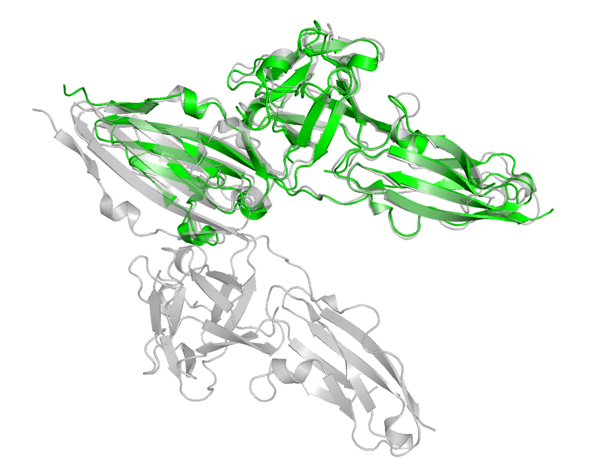
This brings an important challenge: selectivity. FGFR2 is part of a family of very similar receptors. FGFR1, in particular, has a structure very close to FGFR2. If we design a binder that only "likes" FGFR2 in a generic way, it may also bind FGFR1. That would be a problem, because FGFR1 has its own normal roles in the body, and blocking it could cause unwanted side effects.
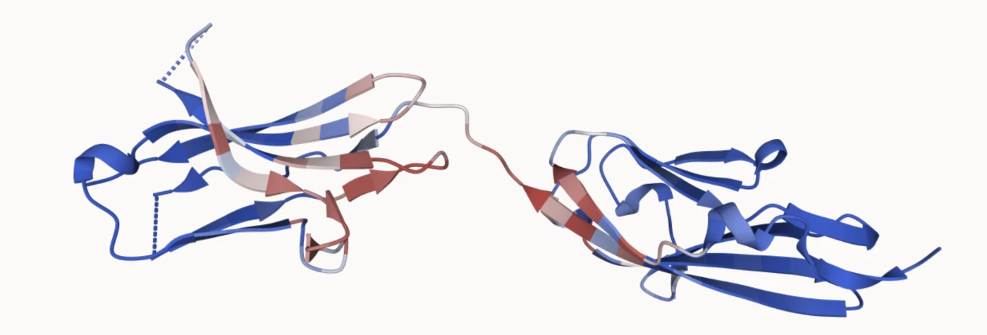
In the structural overlay below, FGFR2 is green and FGFR1 is gray. They share substantial structural similarity, which means the binder choice has to be specific rather than merely sticky.
Let us now put it on the quantitative side for ML. When designing a binder, we can use a number of affinity measures to estimate how well it binds to the target protein. The chosen metric for this hackathon was iPSAE, a confidence score for protein-protein binding. Our goal was to maximize iPSAE between our designed binder and FGFR2, while minimizing the same score with respect to FGFR1. This is commonly called minimizing the off-target binding.
We will talk later about the models and tools we used to generate protein binders and measure iPSAE, but at this stage of the hackathon, after figuring out the main problem, it was time for our biology teammates to shine. A crucial step was figuring out which regions of the target our binder should attach to, and making principled choices grounded in protein biology.
Design choices
The first priority was to clarify the key design choices: which specific regions of the target the binder should engage, and which ML tools we could use to generate it. With less than 48 hours available, this step is critical. There is not much time to iterate through many trials. Generating batches of targets takes time, and we wanted to generate large batches to maximize the probability of getting at least one good binder.
At this point we decided to split based on expertise: the biology people identified the target regions, while the ML people set up the model pipeline and made sure it worked. During this phase, constant dialogue matters. While choosing the biological constraints, you must make sure you have models that can satisfy them. This is also how you learn a lot about the biology side of the problem; most of what I am writing here I learned during the hackathon.
Identifying the target
When designing our binder, we first had to decide which part of FGFR2 to target.
This was important because FGFR2 is very similar to other receptors in the same family, especially FGFR1. Our goal was to find a region that satisfied three conditions.
- It had to be exposed, so a binder could physically reach it.
- It had to matter biologically, meaning it should be involved in receptor recognition or function.
- It had to be different enough from FGFR1, so the binder could learn FGFR2-specific features.
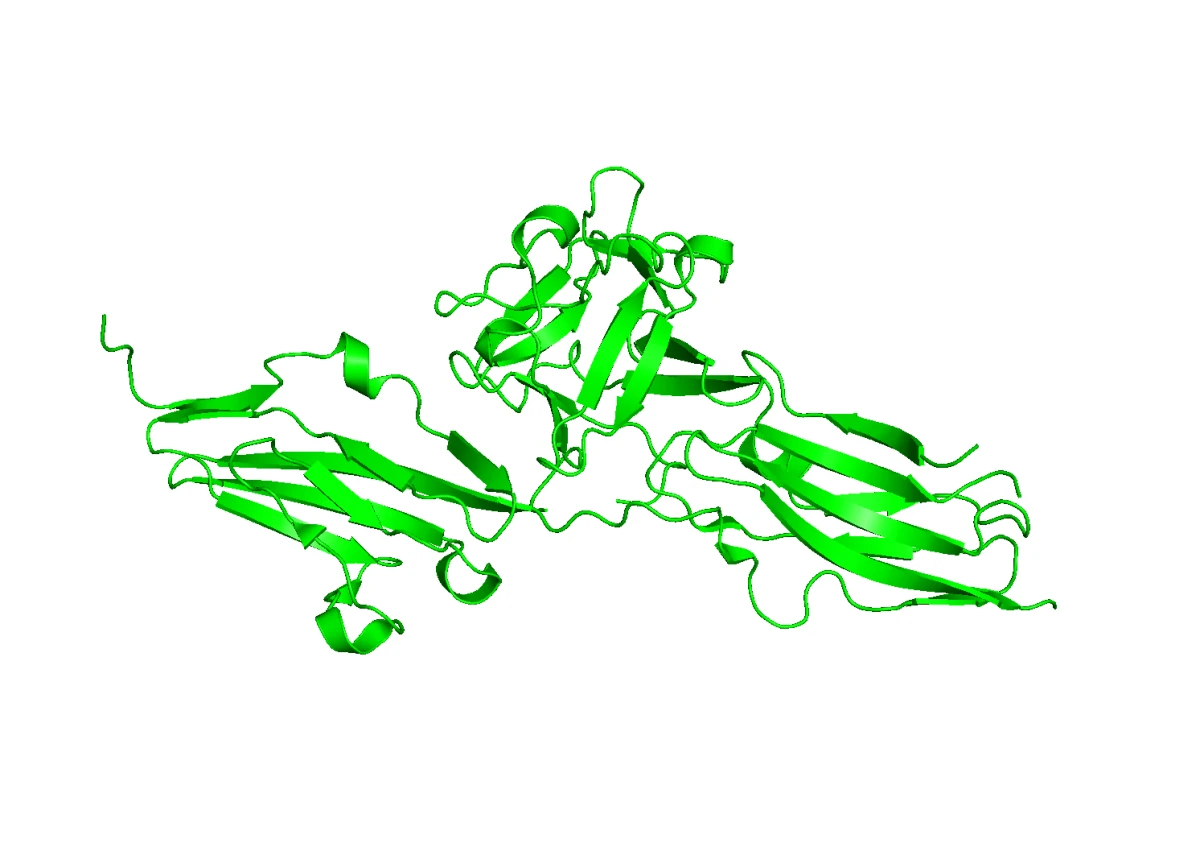
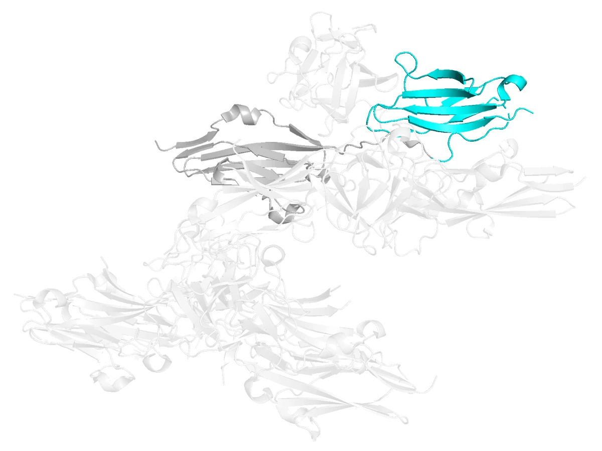
Based on structural inspection and sequence comparison, we selected the D3 domain of FGFR2. This domain is part of the extracellular region of the receptor and contributes strongly to ligand specificity.
More importantly for our design task, D3 contains exposed loops and variable residues that differ between FGFR2 and FGFR1. These differences give the binder something specific to recognize.
After identifying a region of the protein to target, we asked whether we could do anything else to improve the odds of getting a successful binder.
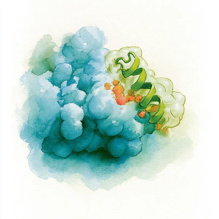
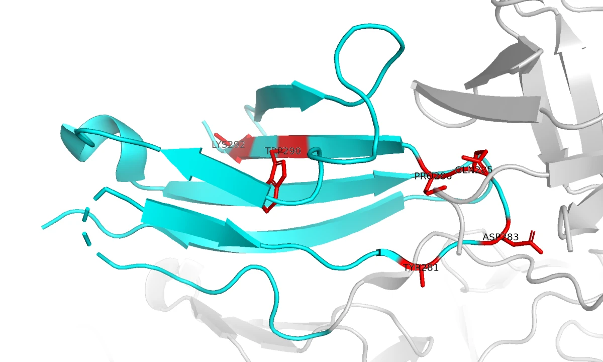
It turns out there are several tools for identifying hotspots: specific residues on the FGFR2 surface that can be used as contact points for the binder-generation model. To choose those residues, we used PESTO, a model that predicts interaction-propensity scores for residues on protein surfaces. This helped us identify surface regions likely to form useful protein-protein contacts. In the image below, the residues in red have the highest predicted interaction probability.
We ended up selecting six residues: 281, 283, 285, 286, 290, and 292.
It was now time to generate a binder.
Choosing the right model
Back to ML duties. The goal was to set up a de novo binder-generation pipeline that could design proteins from the input specifications we identified.
You will most likely be given some basic resources, but if you have access to a good GPU server, use it. Setting everything up can consume some of your initial head start, but it is a huge advantage in the long run. One fundamental choice is which model to use for binder design. There are many possible candidates, but here are some lessons we learned.
- There are many models for de novo binder generation, but none of them is perfect.
- BindCraft can generate high-quality binders, but it is slow. We discarded it because the time budget was too tight.
- RFDiffusion is strong at generating binder backbones. It was a real option, but we chose a more straightforward route.
BoltzGen looked like the best overall decision. It handles structure prediction and binder generation, accepts specifications through a clean YAML file, and includes quality scoring for generated proteins. The binder-generation phase is not too slow, and you can either set up the open repository on a server or use the BoltzLabs platform. If you want to learn more about BoltzGen, here is a related post I wrote on it.
Once you make sure you can generate at least one complete sample protein with BoltzGen, write the YAML config and pass it to the model pipeline. In our case, the YAML looked like this:
# FGFR2 target structure.
# Put the prepared FGFR2 mmCIF/PDB here.
- file:
    path: fgfr2_target.cif

    # Target chain is E.
    include:
      - chain:
          id: E

    # FGFR2 D3-domain hotspot patch selected from our analysis.
    binding_types:
      - chain:
          id: E
          binding: 281,283,285,286,290,292

    # Keep the target structure fixed/specified.
    structure_groups: "all"
Then generate a batch of proteins. The more you can get, the better. Given the time available during a hackathon, you might generate a few hundred proteins, but ideally you would generate thousands. This highlights another point: it is also a game of luck. Models are not yet perfect. Generating many thousands of proteins is partly about trying to win the sampling-space lottery.
Evaluating generated binders
BoltzGen already has a ranking pipeline built in. After generation, it refolded each binder-target complex using Boltz-2 and computed a set of metrics: pTM/iPTM, PAE, refolding RMSD, hydrogen bonds, salt bridges, buried surface area, and more. Hard filters remove the obvious failures first, then surviving candidates are ranked across all metrics using a worst-rank strategy, meaning a binder has to be decent across the board rather than great on only one metric. We kept the top five designs by iPSAE.
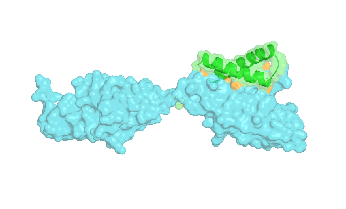
iPSAE is the key metric here. It is Boltz-2's confidence that your binder and target are forming a real, structurally sensible interface. Higher is better.
But a high iPSAE on FGFR2 means nothing if the binder also latches onto FGFR1. So we ran a second round of Boltz-2 predictions to measure off-target iPSAE. The setup was simple: feed Boltz-2 a two-chain input, your binder sequence plus the FGFR1 sequence from PDB structure 1FQ9, and let it predict whether a real interface would form. Low off-target iPSAE means the binder probably ignores FGFR1, which is exactly what we wanted.
In our case we ended up generating the best overall binder of the hackathon, with an iPSAE of 0.7 for the target and 0.1 for the off-target protein. The numbers indicate both good predicted binding to FGFR2 and high specificity, since the predicted affinity to FGFR1 was close to zero.
Did we solve cancer?
We did well, but the metrics are only theoretical until tested in the lab. A fundamental thing to remember is that scores like iPSAE are proxy metrics produced by models. They are not direct measurements of binding affinity. iPSAE tells you how convinced Boltz-2 is that a real, structurally coherent interface would form. It is only as trustworthy as the model generating it.
Models like Boltz-2 are not neutral observers. They are trained on existing structural data, which is skewed heavily toward alpha-helical proteins. Beta-sheet rich structures, for example, are underrepresented, and the model may therefore be systematically less reliable when scoring or generating them.
As a bonus, both for a hackathon and for real experimentation, it can be worth measuring other properties of the generated binders. In our case we used ImmunoGeNN to estimate immunogenicity risk, splitting each protein into overlapping 15-mer peptides and predicting population-level MHC-II presentation risk.
That is just one example of a broader principle: a growing ecosystem of specialized models lets you probe almost any property you care about computationally before touching a pipette. Solubility predictors can flag sequences likely to aggregate. Thermostability models estimate how well a protein will hold its fold under physiological conditions. Others can predict expression levels, half-life, or susceptibility to proteolytic degradation. None of these replace experimental validation, but layering multiple in silico signals gives you a richer picture of your candidates and can save a lot of lab time by deprioritizing binders that look problematic early.
We must have won, right?
No. And this is one of the major take-home lessons from this hackathon. In this kind of event, scores are only half of the story. The other half is how you present the work. You need to create a pitch around the project and sell the idea.
What counts is telling a story, and most importantly, talking about the future. While other hackathons may have straightforward monetary or product metrics, in this case it helped to state clearly how the project could move from computational design to wet-lab validation.
We fumbled this part because, from our internal evaluations, we believed we would not make the finals. We dedicated too little time to the presentation, convinced it would not matter. Final lesson: keep pushing until the end, and remember that when evaluations are not public, there is always an opportunity to turn the result around.
I hope this was a useful logbook of this hackathon. We are witnessing a remarkable shift in the bio domain. We are at a point where it is possible to experiment with disease-relevant targets with only a table, caffeine, and less than 48 hours. I also hope I have shown some of the current limitations of these models, and I think there is still a lot of work to do.
Keep pushing the field.